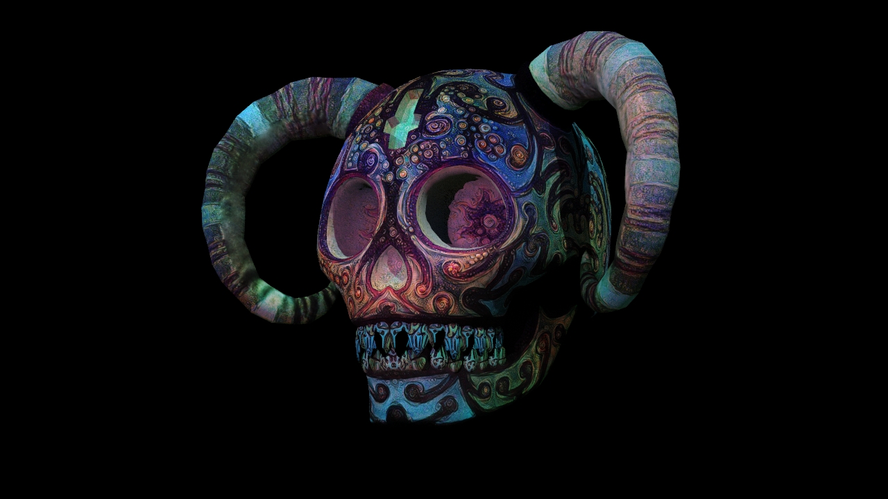
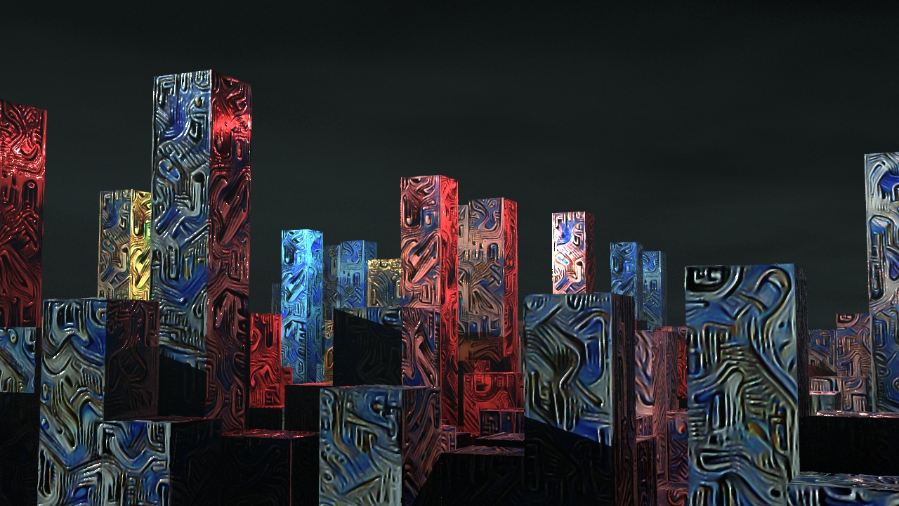
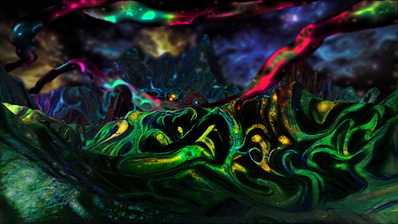
Federico Ferlito | 3D Style transfer

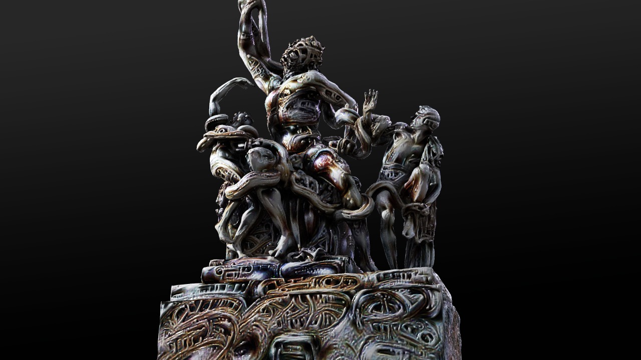
Neural networks have been very popular in the last years, especially in the field of computer vision, where they achieved remarkable results in tasks like image classification. In the last years, a new wave of artist is pushing their bundaries further, using techniques like DeepDream, style transfer and feature visualization to create artistic images and abstract visualizations.

All these technologies are based on the same intuition. Convolutional neural networks are formed stacking layers of artifical neurons. These layers can interpret the input images as they store some abstract representation in their parameters (called weights) using an operation called convolution. These representation are stored in layers that we call feature maps. Once we feed an image to a network, each pixel will contribute to the activation of certain feature map, which in turn will lead to a certain prediction. We can use these representation in a different way: to describe some properties (a.k.a. style) that we want to optimize in a picture. This optimization is possible as the activations each filter are differentiable with respect to the input: this means that we can tweak the input using the gradient descent (or other algorithms) in an iterative way.

An example of such application is called neural style transfer, an optimization technique used to achieve image stylization in a non-photorealistic way. In the next sections, the basic concept of style transfer is described. Following, an extension for applying this technique on 3d models is given.

Neural style transfer

Neural style transfer is used to take two images, a content image and a style reference image (such as an artwork by a famous painter), and blend them together so the output image looks like the content image, but “painted” in the style of the style reference image. Some examples of stylized images are shown below.

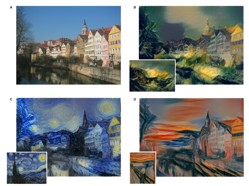
Example of style transfer, taken from the original paper. In the top left image, there is the content. In the three other images, the output for three different styles is shown.

The main architecture requried for style transfer is a pretrained convolutional neural network. Then, the optimization procedure is computed using three components: (i) a content image, (ii) a style image, (iii) and the input image, which is the one that is generated as final output. What allows the network to generate these beutiful stylized images is at the core of the optimization process: the loss function. Let’s discuss them in detail to understain better what’s going on.

A matter of loss

Neural style transfer is based on two loss functions: the content loss and the style loss. The first ensures that the activations of the higher layers of the neural network activates in the same way between the content image and the generated image. The other loss allows the correlation of the activation between the layers on the networks are similar between the style image and the generated image. Let’s break each of the functions down.

Content loss function

The content loss function allows that what it’s represented in the content image to be preserved in the generated image. It does so based on the pattern of activations of the last layers of the model. The different layers of CNNS captures patterns with different levels of detail: the first layers focus more on the individual pixels, and they learn small patterns like lines or curves. Deeper layers of the network learns more abstract shapes. Below, we can see how the different filters activate when the image of a face is fed to a CNN.

Filters of the CNN at different level of depth learns features with different complexity: first layers learnt basic primitives (edges and colours). Deeper filters learnt textures and patterns. The final layers contains complex features, which can resemble objects from the training data.

Therefore we will use the pattern of activation of the last layer of the CNN to define this loss function. Let A be the activation of a layer l, at the i-th feature map and the j-th position. Then the content loss function, based on the generated image g and the content image c, is defined as:

$L_{content} = \frac{1}{2} \sum_{ij}^{} (A^l_{ij} (g) - A^l_{ij} (c))^2$

In a nutshell, this function takes the root mean squared error between the activation produced by the two images.

Style loss function

Defining the style loss function requires some extra steps than the previous loss. In order to extract the style from the CNN, we make use of all the layers available. We then define the style information as the amount of correlation between the features maps in a given layer. The loss is then defined as the difference in correlation between the feature maps activated by the generated image and the style image:

$L_{style} = \sum_{l}^{} w^l L^l_{style} \qquad where \\$

$L^l_{style} = \frac{1}{M^l} \sum_{ij}^{} (G^l_{ij} (s) - G^l_{ij} (g))^2 \qquad where \\$

$G^l_{ij} (I) = \sum_{k}^{} A^l_{ik} (I)A^l_{jk} (I)$

Where w is a weight given to each layer during the loss computation and M is a hyperparameter that depends on the size of the layer l.

Even though the formulas above seems complex, the idea behind is very simple. The goal is to compute two style matrices, one for the style image and one for the generated image. Then, the loss is defined as the root mean square difference between the two style matrices. The style matrix (also known as Gram matrix) captures the distribution of features maps in a given layer. Minimizing the style loss between the two images, we are trying to match the distribution of features between the two images.

Final loss

The final loss is defines as a weighted sum of the two losses defined above:

$L = \alpha L_{content} + \beta L_{style}$

Where α and β are two hyper-parameter decided by the user. Controlling these two parameters allow to control the amount of style and content injected in the generated image. In the examples below the effect of these two parameters is shown.

Example of style transfer for different values of α and β, taken from the original paper. In the left, the ratio α/β is the smallest: the generated image contains mostly the pattern of the style. As we go to the right, the ratio become bigger, and the pattern of the content image appears more clear.

Changing the parametrization of the optimization problem can change drastically the results of the neural network, despite the other components (i.e. loss function) remains the same.

3D Neural style transfer

Example 2

Example 3

Example 4